Flipping Flapjacks, Pruning Pancakes, and Depth First Steps

In the previous post in this series I spent some time trying to convince you that toy problems are worthy of your attention. In particular, I tried to sell you on the notion that the pancake problem was worthy of your attention.  It isn’t necessarily because flipping flapjacks is in of itself fascinating.  It’s because the pancake problem is a relatively simple test-bed for evaluating combinatorial search algorithms like depth first search.  It’s easy to describe, it’s easy to visualize, and it’s easy to scale to comical sizes.

I further argued that combinatorial search algorithms are interesting because they’re so general.  Specifically, I said, “I think that combinatorial search is useful tool to have in your bag because i think that problems like ‘find me the cheapest X in Y’ come up not infrequently.” I want to be a little more specific about that now.  We’re going to work through a series of domains of decreasing silliness. Further, it’s reasonable to approach each of these problems as a search problem. The problems are:

• How do I efficiently order a stack of pancakes?
• How cheaply can I visit every Dunkin’ Donuts in the continental US?
• What’s the best schedule for interviews between some students seeking internships and some companies seeking interns?

At the end of  the last article, I laid out some learning goals.  In this article, we’re going to focus on the following two points:

• Understand what makes a problem a combinatorial optimization problem
• Master a basic tree search technique (Depth First Search)

The Pancake Sorting Domain

Domain Terminology:

• Action – Something you do in the domain- E.g. flip the pancake stack
• Solution – A way of achieving something, typically a list of actions
• Problem or Instance – A thing you want to get a solution for
• Domain – The thing from which a problem might come- E.g. Pancake Sorting, that’s the domain here.
• State – A situation in the domain- E.g. particular ordering of pancakes
• An instance is often described by its initial state
• Goal – The thing we want to achieve- E.g. The pancakes are ordered

The pancake problem, or pancake sorting, asks us to figure out how to efficiently order a stack of pancakes by size using a spatula. Imagine you’re serving pancakes up to some friends for breakfast.  Unfortunately, you’re imperfect and so are your pancakes: they’re all of different sizes! To make your pancakes as pleasing as possible, you decide to plate them in order from largest to smallest. This way they form a little ziggurat, as we see in the Figure above. That ziggurat is your GOAL.

Now, that’s already a little comical, but it gets better. You’re going to refuse to dirty another dish now that you’ve got all of the pancakes out of the pan.  In fact, the pan is already soaking, so you can’t even use that for staging. Further, you refuse to lay a finger on the flapjacks directly. You can only manipulate the stack by inserting your spatula, and flipping the whole stack above it. Selecting where to stick your spatula and flipping the stack above it is your ACTION.  The above Figure shows us putting a spatula underneath the second pancake in a stack.  Flipping the pancakes above the spatula in this image would produce a goal.

So, let’s say that the Figure  above shows the stack of pancakes you produced by stacking them up as you come out of the pan.  This is both a STATE as well an INSTANCE, because it happens to be the initial state of the problem. A SOLUTION takes the form of a series of actions, that is locations to put the spatula and flip the stack, that converts the stack in that Figure into the ziggurat we saw early.  The solution is shown below:

An Implementation of the Pancake Domain

We’ve just described the pancake problem, and we took care to **CALL OUT **the parts of the domain definition that are crucial for search. Now let’s take a look at each element in detail.  We’re going to see how we represent the pancake problem in F#, one piece at a time. At the end, we’ll see how that implementation aligns with a domain model that can be handed to a search algorithm in order to get a solution back.

State, Instance

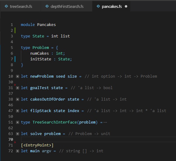
The figure above shows how we represent the pancake problem in F#.  On line 3 we declare that we’re going to be representing stacks of pancakes as integer lists.  When we set up the problem, we said that all of the pancakes were of different sizes.  A list doesn’t enforce that constraint; you’d need an ordered set for that.  I’m trying to split the difference between having something that lets the compiler enforce our domain model and something that’s easy to write and read, erring towards the side of ease of use. So, I used a list rather than a set and we’ll have to be careful to only construct instances with unique elements when making problems.

Lines 5 through 8 define pancake problems.  They’re just states with a little bit of extra information: the number of pancakes in a stack.  State and problem could have been identical here, but as we’ll see shortly, the number of pancakes in the stack is something we ask about frequently.  Rather than ask for the length of the list that is the state repeatedly, we pack it into a record along with the initial state so it’s easy to look up.

Actions

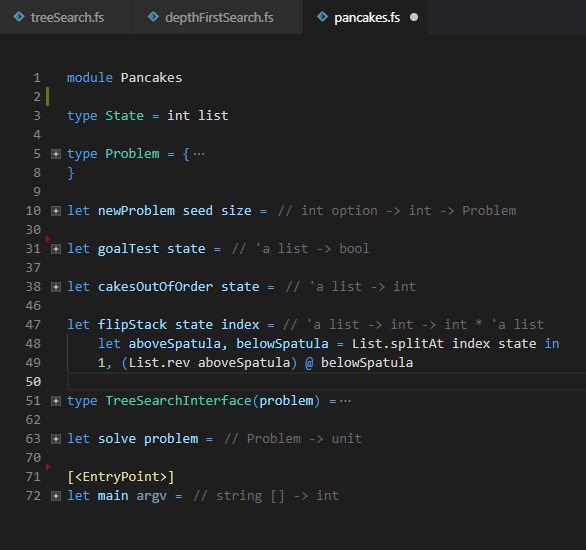
When defining the pancake problem, we said there was a single action: sticking your spatula into the stack and flipping the top half of the stack over. We see that modeled above.  First, we split the state into two parts based on the index of the spatula.  Then, we return two things:

• The cost of the action
• The state that results from the action (we reverse the prefix of the list and then concatenate them back together)

Remember that we’re trying to find the most efficient approach to stacking these pancakes in order.  That’s why the cost plays an important role.  For the pancake problem, all actions have the same cost, at least in our model. This is often referred to as being a unit cost domain.  The problems we’ll look at in the future will have more interesting cost models.  The cool thing about search is that, so long as we report the cost along with the new state that results from the action, we don’t have to change anything about our solvers when we swap the domain out from under them.

Goals

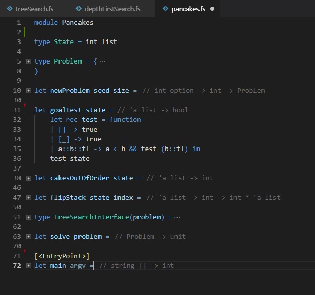
Finally, we define a goal test for the pancake problem.  Earlier we said that a state was solved, or a goal, when all pancakes in the stack were in order.  There are a lot of different ways to define an in-order test for a list in any programming language, but we chose the following:

• The empty list is in order by definition.
• So is the list with exactly one element.
• Any list is sorted if its first two elements are sorted and all elements from the second on are sorted too.

I picked this implementation for pedagogical reasons (there are more efficient tests): This test uses recursion and pattern matching; I wanted a simple example of those before they start to come up in complicated ways in the search code.

Hey, I saw some other things you didn’t expand in that code…

Yup. You saw random instance generation, which isn’t particularly interesting for describing domain modeling or problem solving.  We just need some way of getting instances to work with for the purposes of this demonstration.  Then, you saw a heuristic (cakesOutOfOrder). We’ll get to heuristics shortly, but I don’t want to talk about them until the very moment we need them. Finally, you saw the TreeSearchInterface, which as you might suspect, how we present the pancake problem as something that a search algorithm can handle. We’re going to talk about that now.

Defining a Problem as a Search Problem

Search Algorithm Terminology:

• Node – Some element in the tree or graph being enumerated- Nodes relate to domain states
• Root – the first node in the tree
• Generate, Generation – Creating a new node
• Expand, Expansion – Creating the nodes that logically follow some given node- E.g. I expanded the root node and generated all of it’s children
• Tree – A collection of Nodes and Edges
• Branch – A portion of the tree
• Prune – To excise a portion of the tree

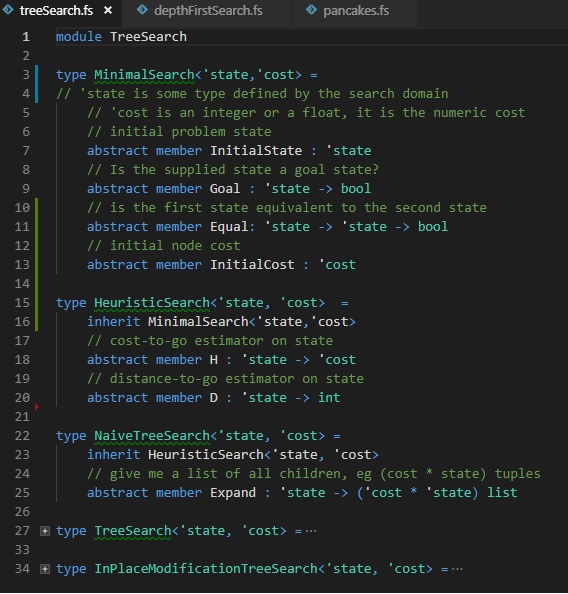
We’ve broken down the interface between the domain (pancakes) and the search code (depth first search) as shown in the code snippet above. We start with a pretty bare-bones definition of a search problem; we need to have:

• Some configuration of the problem
• A goal test
• Some way of seeing if states are the same
• An initial cost value

Why did you put cost in there?

That last one might seem a little weird, but I want to be as abstract as I can be about the cost of a solution to a problem so that the algorithms I define are as general as possible.  The pancake domain has integer cost, but other problems may have costs which are floats, or which are stored as rational and irrational components.  That’s how you’d think about 8-directional movement on a grid (integer costs for cardinal directions, multiple of square root of 2 for the ordinal directions). Sometimes you run into multi-objective optimization problems where cost is actually a vector of incomparable features.  The idea is that, while it may be critical for the domain to care about such things, the search code does not have, nor should it (save for performance arguments, perhaps).

What’s a heuristic?

Next, we refine the search down to a heuristic search.  We need at least those elements that we had to define the previous search, and then we add in heuristics.  Heuristics are estimates of some important domain property.  Here, I’ve restricted our heuristics to h, the common abbreviation for cost-to-go, and d, the common abbreviation for decisions-to-go.  Cost-to-go is, as one might expect, an estimate of how expensive the problem will be to solve from a given state. In the case of the pancake problem, this means exactly “how many times will I need to flip the stack between here and a goal state”.  Decisions-to-go is how many states lay between the current state an the goal.  Since the pancake problem is unit cost, these are the same for our domain.

Expanding on Expand

Finally, we expand heuristic search into NaiveTreeSearch. We need one last thing to perform any kind of search on these problems. We need some way of taking a problem state and getting all of the adjacent problem states.  The expand function is a little more complicated here because we return a list of adjacent states and the cost of reaching them. This is, again, just an attempt to keep the solvers as general as possible.  You might notice this is really close, but not identical, to the type signature of flipStack in the domain code.  flipStack makes one state, here we need to make them all.

Hey, I saw some other things you didn’t expand in that code…

Yup.  You saw some more advanced tree search interfaces.  It turns out that the simplest approach isn’t sufficient for many problems you might care about.  It isn’t even enough for the pancake problem if you want to solve really, really big instances of it.  We’ll see why next, when we start looking at and evaluation search code.

Marrying the Domain and the Search

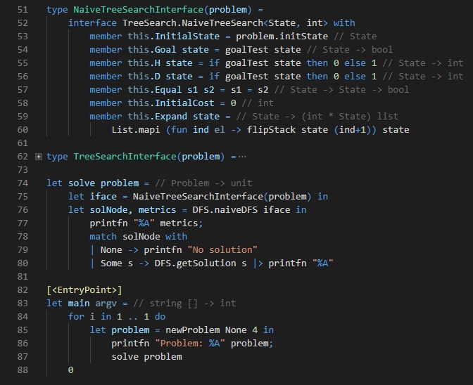
The above is meant to close the loop between the search interface and the domain itself.  From lines 51 to 60, we define a search problem in terms of the pancake problem. On line 51, we say that the search interface is derived from a problem instance. On line 53, you can see why — the search interface provides the initial problem state.  Thus, it has to be instance specific. While the goal test (line 54) is unremarkable, the heuristic functions are a little funny in that they’re defined in terms of the goal test.  We’ve given the search the simplest imaginable heuristic: if the problem is not solved already, there must be one more step at least. Equality (line 57) is simply equality on integer lists. The initial cost is 0 (line 58).   We get a little cute with the expand function: we imagine putting the spatula into every gap between pancakes (or pancakes and the plate in the final case), but we do so by mapping over the elements of the current stack of pancakes. The effect is that we produce a list of successor, or child, states to a supplied state, along with the cost of reaching them, which is always 1 here.

Lines 74 through 80 invoke depth first search on the problem.  Lines 83 through 88 are the program entry point, where we set up some problems and solve them.  We’ll talk about depth first search as a solving technique shortly, but we should spend a little time discussing the domain-as-search approach here. Now we’re going to look at depth first search purely in terms of the supplied search interface.

Depth First Search

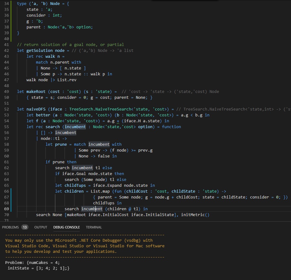
Code (and results; we’ll get to them) for depth first search are provided above.  Lines 34 through 38 define a node for the search algorithm.  A node has a cost of reaching it, g, a state that it describes, and a parent. The parent can be Some other node, or it can be None in the case of the root of the search (hence the option).  Lines 42 through 47 show how we convert a given node, assumed to be a goal, into a solution: we follow parent pointers up to the root and then reverse the list.  This gives us the states leading to the solution in order.  You could compute the actions in the solution from here, or you could store the actions along with the states directly.  We chose the former because it allows for some convenient pretty-printing and debugging. Lines 49 and 50 show how to build a root of the search problem from an initial problem state.  Finally, lines 55 through 70 describe a text-book implementation of depth first search.

A Search Iteration

Line 55 is the top of the function call.  We see this is actually depth-first branch and bound, and not just plain old depth first search, by the first argument, incumbent.  Incumbent is short for incumbent solution, and it represents the best answer we’ve found to date.  We’ll be careful to only record improving solutions, and we’ll use the incumbent as a bound for pruning potential branches of inquiry (that’s why it’s branch and bound!).

The second argument (Sir Not Appearing in this Sugaring) is the list of all nodes we need to consider, which I will call *open *or maybe stack since this is a tree search.  It starts out as [ root ] in line 70.  First, we ask if the open list is empty (line 56).  If it is, great, search is over, as there’s nothing left to consider.  Incumbent is the provably optimal solution to our problem, and we return it. If there are some nodes left to consider, then we start thinking about them.

Pruning

The first thing we do is split the open list into its first component, node, and the other components, *tl *on line 57.  The first thing we do is we decide if node is worth considering at all. If there’s no incumbent (line 60), we know we have to consider this node.  If there is some incumbent, we ask if the cost of the incumbent must be smaller than the cost of the node (line 59).  Prune is only true if there is an incumbent whose cost is less than the lower bound of the cost on a solution passing through node. We compute that bound, as seen on line 54, as *node.g + (H node.state). g *is the cost incurred getting to the node; in this specific case it is equal to the depth of the node in the tree and the number of spatula flips we’ve done. H is a little hairier. It’s a lower bound on the number of flips we must do in order to solve the problem.  Right now, it’s equal to 1 for all nodes which are not at a goal state, because that’s a really cheap-to-compute lower bound.  We’ll talk about how better lower bounds improve performance next post.

New Goals

Once we’ve decided if this node should be pruned, we act on that decision (line 61).  If we prune the node, search simply continues on the remainder of the open list.  If the node looks promising, the next thing we ask is if it is a goal.  If the node  is a goal, we know it’s better than the previous incumbent: node.g < Incumbent.g by virtue of the fact that H node.state must be 0 and node wasn’t previously discarded.  If it’s a goal, we continue searching with this new improved incumbent (line 64).

Think of the Children

If the node isn’t a goal, we need to make sure we consider all of its children.  Remember last week when we saw others describe combinatorial optimization as “a topic that consists of finding an optimal object from a finite set of objects”? Well line 61 makes certain we converge on the optimal object, and lines 65 through 68 make sure we enumerate every element in the finite set of objects.  All of the possible child nodes are computed as children on lines 66-68. Then, we continue search, with the children we just generated put on to the front of the open list.

Evaluating Naive DFS

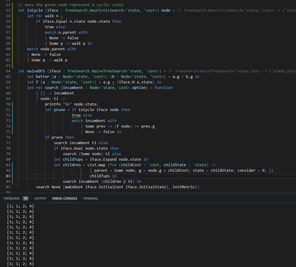
Hopefully, you’ll have noticed that there’s no output that comes out of DFS here, despite the fact that we’re guaranteed to enumerate the whole space and find the optimal solution.  If we add a little instrumentation to the search (that is, if we print every node we visit, as we do on line 70 above) the problem becomes immediately apparent. We keep visiting the same states.  That’s because the pancake problem contains cycles. That is, you can revisit a state of the problem by simply applying the actions that define the domain, like say flipping the top pancake and only the top pancake, or inserting your spatula into the same index twice in a row.

Look Ma, No Cycles!

There is balm in Gilead, and it is found on lines 52 through 62, which implements cycleDetection.  We’re going to make sure that no path visits the same state twice, and if it happens to, we’ll prune that branch of consideration (prune is updated in lines 71 through 75).

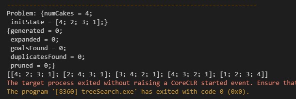
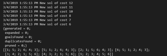
Now, the output which we saw above is much better — we actually get a solution! It happens pretty fast, which is also very cool.  There’s only one problem: I’m a very hungry guy, and there’s just no way that four pancakes can satisfy. Let’s say, for sake of argument, that I need at least 6 pancakes before I’m full.  We run the solver again.  We generate a few hundred solutions in the course of a second and find a very quick way to serve up a stack of six pancakes, as we see below.

But I’m still hungry…

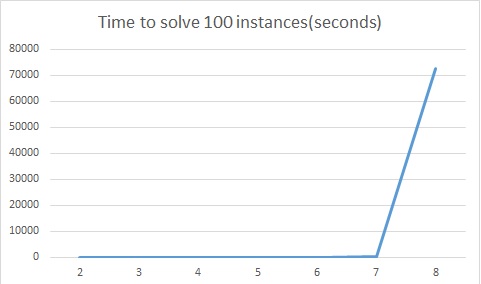
But wait, I said we were plating pancakes for a group of my friends!  Six can’t serve us, we’re going to need at least 30 pancakes for my retinue. Here’s where we run into the problem with combinatorial search — it’s super expensive.  The depth first search we just implemented can find solutions to the 30 pancake problem (or the N-pancake problem for arbitrary N). It’s just a question if you want to wait that long.  First, there’s the practical consideration of the hotness of our hotcakes.  We want to serve the pancakes before they cool, and solving the 30 pancake problem this way can take several days if you want the best solution.  The figure above shows the scaling performance of our pancake solver up to N=8 pancake stacks (cumulative time to solve 100 instances).  We’re doing pretty well up to 6 pancakes.  There we can solve instances in fractions of a second or seconds at most.  We start to need hundreds of seconds in the 7 pancake problem.  When we hit 8 pancakes, we need around 20 hours to solve 100 instances.  That’s just too long on average to think about how to plate the pancakes.

Second is the practical concern of our own mortality.  Maybe you and yours don’t mind cold pancakes.  Maybe you think you’ll just wait until the algorithm returns and then plate them up after they’ve cooled.  The issue is you’ll probably die first.   The way we’ve represented the pancake problem induces a tree with branching factor equal to the number of pancakes, in this case, 30.  If we just do some quick ballparking, without considering things like cycle detection, the uneven depth of solutions, and so on, we would expect to see 30^{avg. solution depth } nodes over the course of our search.  For the sake of argument, let’s assume we only need to explore a tree of breadth 30 and depth 10, inducing 30^10 = 5.9049e+14 search nodes.  If we tuned the code to touch 100,000 nodes a second, we would still need a little over 187 years to see the optimal solution using this approach.