DIY AI: Sentiment Analysis P2: Implementation

Blog Post Written By: Lisa Lo

Once again, we’re back to discuss sentiment analysis. In our last post, we went over what sentiment analysis is, why it’s useful, and the main approaches to solving sentiment analysis. Now, with all that knowledge in hand, it’s time to start coding our own sentiment analyzers!

Setup

You’ll need to have a coding environment with the following installed and configured:

If you need help setting up python, check this guide out!

Otherwise to add these libraries, run:

pip install textblobpip install vaderSentimentpip install nltk

We’ll be going through two different ways of creating a sentiment analyzer:

Using pre-existing libraries and calling their sentiment analyzers
Using nltk to create a supervised learning based analyzer

Some experience with coding will be needed (or prepare for lots of googling); but otherwise let’s get down to it.

Pre-Existing Libraries

If you’ve been developing in Python for some time, you probably know there are libraries for almost everything. Sentiment analysis is no different. While there are many different libraries handling sentiment analysis and various portions of it, two of the most well known ones are TextBlob and vaderSentiment. These libraries are especially nice because they perform the sentiment analysis for you. All you need to do is pass in the text, and they return back information that translates into sentiment. Moreover, vaderSentiment is especially known for its ability to handle social media speech since it was created with that in mind.

Now I promise that in three minutes you’ll be able to find the sentiment of sentences. Ready?

from textblob import TextBlobsentence = "Hey, I'm a great sentence!"text_blob_sentence = TextBlob(sentence)text_blob_result = text_blob_sentence.sentimentprint(text_blob_result)from vaderSentiment.vaderSentiment import SentimentIntensityAnalyzersentence = "Hey, I'm a great sentence!"vader_analyzer = SentimentIntensityAnalyzer()vader_result = vader_analyzer.polarity_scores(sentence)print(vader_result)

Run these two scripts and voila, we have sentiment analysis going!

To use TextBlob, we created a TextBlob object for every piece of text. This TextBlob object automatically stores the sentiment, which we then retrieved.

For vaderSentiment, we created an instance of a SentimentIntensityAnalyzer. From there, any text can be passed into the polarity_score method of a SentimentIntensityAnalyzer instance.

Let’s take a look at the results.

Text Blog Output: Sentiment(polarity=1.0, subjectivity=0.75)Vader Output: {'neg':0.0, 'neu':0.345', 'pos':0.655, 'compound':0.69}

Textblob returned polarity and subjectivity. Polarity is an extremely common term used to reference how negative or positive text is. In this case, its value ranges from -1 (negative) to 1 (positive). Subjectivity explains how much of the statement is fact versus based on opinion. 0 is hard fact and 1 is essentially opinion.

Figure describing the strength of sentiment being either positive or negative.

Combining the two gives us a clearer picture. If a statement is ranked with a low subjectivity and near 0 polarity, it’s probably a neutral statement. Alternatively, with high subjectivity and with low or high polarities, there are likely some fiery tempers backing it.

From Vader we got four outputs: ‘pos’, ‘neg’, ‘neu’, ‘compound’. Pos, neg, and neu show how much of a sentence is positive, neutral or negative. So, these scores add up to 1.

The compound score represents the same thing as the polarity score from TextBlob. It gives a weighted sum of all the parts making up the sentence which is normalized to give an output between 1 (positive) and -1 (negative). A general measure of determining overall sentiment is: a compound score of above 0.5 is positive, less than -0.5 is negative, and anything else is neutral. Sometimes more specific ranges like -0.1 to 0.1; or an offset is a better choice. Still, you could also use the composition of the sentence saying that if any of this sentence has negative words than it’s negative. Ultimately, it’s up to you to make the final call using these measures.

With all of this, a very simple method for getting definite polarities for TextBlob would be:

def get_definite_polarity(text_blob_result):    # 0 is negative; 2 is neutral, 4 is positive    subjectivity = text_blob_result['subjectivity']    polarity = text_blob_result['polarity']    positive_threshold = 0.5    negative_threshold = -0.5    if subjectivity == 0:        return 2    elif polarity > positive_threshold:        return 4    elif polarity < negative_threshold:        return 0    else:        return 2

and for Vader it’d be:

def get_definite_polarity(vader_result):    # 0 is negative; 2 is neutral, 4 is positive    compound_score = vader['compound']    positive_threshold = 0.5    negative_threshold = -0.5    if compound_score > positive_threshold:        return 4    elif compound_score < negative_threshold:        return 0    else:        return 2

From here, you can play around with the positive and negative thresholds till you get the result you want!

Vader (and maybe Textblob) use a rule-based approach to solving sentiment analysis. This has the advantage of not needing training data as well as speed. Moreover, because they had several people dedicted to creating these systems, they could integrate many of the common patterns found in text speech resulting in reatively reliable accuracy.

Again, this supports how rule-based systems are great, just time-consuming to create on your own, thus it’s great to search out already built ones.

Now, we have something quickly turning over (or outputting a result); however, you may want more control or even want to understand how sentiment analysis works from a deeper level.

To better understand what these tools do, let’s try rolling our own.

Supervised Learning

Supervised machine learning is well suited to sentiment analysis given how much data there is out there. There are lots of examples all over the web of positive, negative, or neutral pieces of text. Feeding it into the computer, we can find what (features) is more likely to appear in the categories of text. Then, when given a new text, it can match and see if the new text has more things relevant to positive, negative, or neutral texts.

So, what’s the what here? Words! Or phrases, or whatever you want. Words tend to be a good starting place. With this basic understanding, we have a map of steps in front of us.

Find a dataset with text labelled as positive, negative or neutral (a polarity value).
Run through each text in the dataset.
Preprocess the text.
Turn every text into a mapping of what words exist in the text (a vector).
Break the processed dataset into a training set and a testing set.
Run the classifier on the training set!

It may seem like a long list of tasks, but it’ll go by in no time! Let’s start at number 1.

1. Finding the Dataset

Social media is a fascinating place so, we’ll be using this dataset (under Where is the training data). Alternatively, there are many other datasets like movie reviews, product reviews, social media records, etc. If you have something specific in mind, there are many web scraping tools that allow you to get the text bodies you want. A word of caution though, you’ll have to label that data (at least if you want it for training and testing). You can always use a different domain to train on; although the accuracy may go down from switching domains. Anyway, download your dataset, and onto step two we go.

2. Run Through Dataset

Run a for loop, now onto step 3! Well, in essence yes, but there’s a little more to it. Take a look at your data file, what do you have?

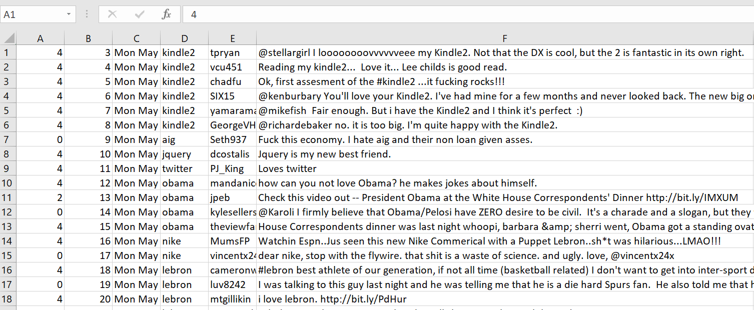
Generally, it’ll open in Excel with several different columns. At the very least, one column should have text and another should have a polarity measure. We need to track which column these are (remember CS 0 indexes everything).

In the Twitter sheet, in column 0 (A) we can see the polarity values with either 0 (negative), 2 (neutral) and 4 (positive). Column 5 (F) shows the actual tweet.

Besides important index values, we also need to keep track of how every column is separated. In a UI like Excel, it’s easy to see, but in reality, the file is a giant text file. There’s a pattern that’s used to showcase when a new column is started and when a new row is started.

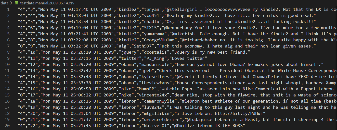
Instead of opening your file through a program like Excel, try opening it with a plain text editor. Here, we see the raw string with a clear pattern: every column is stored in quotes, and separated by a comma. A new row is a new line.

Now we have 3 key pieces of information:

Which column indexes are relevant
What character (or sequence) marks a new column
What character (or sequence) marks a new row

We’re ready to start coding.

path = 'twitter_data.csv'with open(path, newline='\n', encoding='ANSI') as file:    for line in file:        line = line[1:-1]        fields = line.split('","')

The path is the name of the data file (I renamed mine). If it’s not in the same folder that you’re working in, make sure to include the folder/file_name in your path!

Here we used ‘\n’ as the newline value since that’s the character representation of how our csv splits different rows. This way, we know line represents a new row.
Similarly we used ‘”,”‘ to split the line up since every column is split by a comma. We cannot use a comma because some columns include commas and we want every element in our list to be an entire column. “,” marks the end of one column and start of a new one; plus it also gets rid of the extra “s around the data.(The line = line[1:-1] also strips away the extra quotes at the beginning and end that aren’t taken care of by the split. )

Now, we have something that reads in a file, goes row by row, and creates a list with each element representing a column in the row.

Here is the next major decision point: what data do we store and how do we store it?

We could choose to store the minimum amount of data: the text and polarity. For the sake of pure sentiment analysis, it’s all we need. Storing the minimum amount of data saves space and keeps everything small and simple. However, in the future, beyond training and creating a sentiment analyzer; you may want to analyze a body of data based on a specific time period, topic, user, etc. When you move beyond the training phase, other data you might find in your datasets can be used to specialize analysis.

For this DIY guide, since we’re not moving beyond creating the sentiment analysis, we’ll stick to the text and the polarity. However, these considerations do effect how we choose to represent the data.

The simplest way to track the data would be a giant list pairing the text to polarity. So we could add dataset = [] before the path declaration; and then after the splittings, add dataset.append((fields[0], fields[5])).

While simple, it’s not super adaptable. What if you want to store more from each row? What if you need more pieces of information associated with each tweet beyond the text and polarity (which we will). You could remove each tweet one at a time from the dataset and then put it back in with the extra information attached, but over time that will get messy.

There are many other ways to approach this problem, but we’ll be creating a class to do so. That way for every tweet we can easily access any information we need; change what we store, and add more information.

class TweetData(object):    def __init__(self, text, polarity=None):        self.text = text        self.polarity = polarity

Going back to what we had before, now we can add dataset = [] before the path and dataset.append(TweetData(fields[5], polarity=fields[0])) after the split.

So, at this point the code should look something like this:

class TweetData(object):    def __init__(self, text, polarity=None):        self.text = text        self.polarity = polaritypath = 'tweet_data.csv'dataset = []with open(path, newline='\n', encoding='ANSI') as file:    for line in file:        line = line[1:-1]        fields = line.split('","')        dataset.append(TweetData(fields[5], polarity=fields[0]))

Step 2 is complete!

3. Preprocessing

Here’s where the heavy work comes into play. With a single word, it carries a lot including but not limited to:

Word transformations: replacing words with other ones (i.e replacing abbreviations with their full words)
Normalization: Making all text appear the same (i.e turning everything lower case)
Tokenization: Splitting text into smaller units (i.e turning sentences into words)
Stemming: Removing prefixes and suffixes (i.e chopping the -ed off words)
Lemmatizing: Reduce words to their base form (i.e ‘am’, ‘are’, ‘is’ all go to ‘be’)
Parts of speech tagging: Identifying the part of speech of every word (i.e adjectives, nouns, proper nouns, verbs, etc.)
Filtering unnecessary words: Removing words that don’t help with the task (i.e ‘a’, ‘the’, etc.)

Not all of these needs to be done; however, they can greatly boost accuracy.

At its core, for sentiment analysis we need to tokenize the text into words, normalize for case, tag parts of speech, and filter out irrelevant words commonly known as stopwords.

Tokenizing text is breaking the text up into the smallest unit, in this case, words. Tokenizing is one of those deceptively simple tasks that becomes infinitely more complicated the more you think about it (Separating based on whitespace is only step one). Luckily for us, nltk already has tokenizers for us so we’ll use that. We’ll also normalize the case, and remove punctuation (you shouldn’t always remove punctuation which will be explained in Improvements, but for now we’ll do so).

def tokenize_words(tweet):    tweet.word_list = []    for sentence in nltk.sent_tokenize(tweet.text):        for word in nltk.word_tokenize(sentence):            word = ''.join(                [character for character in word if character.isalnum()])            if word != '':                tweet.word_list.append(word.lower())

nltk.sent_tokenize separated the text into its sentences, and then nltk.word_tokenize seperated the sentences into words. For each word, we went character by character, taking out anything that’s not a letter or number, then lowercased the word. You can also choose to do stemming and lemmatization before we add the word into the word_list for that tweet.

lemmatized_word = nltk.stem.WordNetLemmatizer().lemmatize(word)stemmed_word = nltk.stem.SnowballStemmer('english').stem(lemmatized_word)

Sometimes these are great to do, but they can also remove information like parts of speech which is why we’ll not use them on our first go.

To add part of speech tagging after completing the word_list:

tagged_word_list = nltk.pos_tag(tweet.word_list)

tagged_word_list will be a list of (word, part of speech tag) and so from there we can decide how we want to filter words out. We want to find the most important words that indicate sentiment; however, if the most frequent word shared is ‘a’, then we’re probably not going to have the best sentiment analyzer. That’s why we want to filter things out. The list of words filtered out is called stop words.

First, let’s look at traditional stopword lists. Nltk already has a stopword list.

from nltk.corpus import stopwordsstopwords.words('english')

If you’re curious what they are, print them out!

['i', 'me', 'my', 'myself', 'we', 'our', 'ours', 'ourselves', 'you', "you're", "you've", "you'll", "you'd", 'your', 'yours', 'yourself', 'yourselves', 'he', 'him', 'his', 'himself', 'she', "she's", 'her', 'hers', 'herself', 'it', "it's", 'its', 'itself', 'they', 'them', 'their', 'theirs', 'themselves', 'what', 'which', 'who', 'whom', 'this', 'that', "that'll", 'these', 'those', 'am', 'is', 'are', 'was', 'were', 'be', 'been', 'being', 'have', 'has', 'had', 'having', 'do', 'does', 'did', 'doing', 'a', 'an', 'the', 'and', 'but', 'if', 'or', 'because', 'as', 'until', 'while', 'of', 'at', 'by', 'for', 'with', 'about', 'against', 'between', 'into', 'through', 'during', 'before', 'after', 'above', 'below', 'to', 'from', 'up', 'down', 'in', 'out', 'on', 'off', 'over', 'under', 'again', 'further', 'then', 'once', 'here', 'there', 'when', 'where', 'why', 'how', 'all', 'any', 'both', 'each', 'few', 'more', 'most', 'other', 'some', 'such', 'no', 'nor', 'not', 'only', 'own', 'same', 'so', 'than', 'too', 'very', 's', 't', 'can', 'will', 'just', 'don', "don't", 'should', "should've", 'now', 'd', 'll', 'm', 'o', 're', 've', 'y', 'ain', 'aren', "aren't", 'couldn', "couldn't", 'didn', "didn't", 'doesn', "doesn't", 'hadn', "hadn't", 'hasn', "hasn't", 'haven', "haven't", 'isn', "isn't", 'ma', 'mightn', "mightn't", 'mustn', "mustn't", 'needn', "needn't", 'shan', "shan't", 'shouldn', "shouldn't", 'wasn', "wasn't", 'weren', "weren't", 'won', "won't", 'wouldn', "wouldn't"]

Looking at the list, you see common words that help sentences flow, but don’t contribute unique information. As a result, they can be tossed.

You might also notice some words that may come in handy like ‘not’. ‘I do not like’ vs. ‘I like’ are two very different sentiments. That’s why there isn’t any “universal correct stopword list”. These are just lists of words that are commonly considered stop words. So, it’s up to you what words from your word_list you wish to remove.

You can always create your own or add to this list if you have other words that similarly don’t affect the sentiment.

def remove_stopwords(tweet):    stopword_list = stopwords.words('english')    stopword_list.remove('not')    new_list = []    for word in tweet.word_list:        if (word not in stopword_list):            new_list.append(word)    tweet.word_list = new_list

Here, we use the english stopwords as our basis, and then remove words that we still think could come in handy. If there’s any other words you think should be stopwords, just add them by using stopword_list.append('word').

Besides words in general, you can also filter on parts of speech! Take ‘apple’ vs. ‘great’. ‘Apple’ doesn’t say anything about how people feel; alternatively, ‘great’ indicates something good! Admittedly, it could be a ‘great disaster’, but either way, it gives us much more insight into the sentiment. As a result, adjectives and other descriptive parts of speech are very important to keep for sentiment analysis.

The list of parts of speech tags are here. Roughly though know ‘J’ is for adjectives, ‘N’ is for nouns, and ‘V’ is for verbs.

def remove_extra_words(tweet):    # type_list = ['J']    type_list = []    new_list = []    tagged_word_list = nltk.pos_tag(tweet.word_list)    for word in tagged_word_list:        if word[1][0] not in type_list:            new_list.append(word[0])    tweet.word_list = new_list

A tag is normally two letters; however by taking only the first letter of the tag, it leaves us with the more general part of speech. Here, we reversed the type_list to be essentially a black list. If it’s in the list, then don’t include that part of speech, otherwise, keep the word.

While not quite sentiment analysis, there is still a lot of interesting information found by looking at nouns or proper nouns. The classifier will end up finding patterns showing subjects and other words that people associate postively or negatively. (Apparently people really don’t like the dentist.) An important thing to remember though is sentiment analysis is about how people feel about something, not the something itself.

Whatever you choose to remove or keep, by the end of this process you should have a list of words. The part of speech tagging would change the list from words to a mix of words and part of speech. In the end, we don’t want to keep the part of speech, we only want the words.

Finally, to bring it all together, we want to perform this preprocessing on everything in the dataset, and also keep a list of all the words from every tweet in the dataset.

all_words = []for tweet in dataset:    tokenize_words(tweet)    remove_stopwords(tweet)    remove_extra_words(tweet)    all_words.extend(tweet.word_list)

If at any point you run into a memory error, this means your training on a set too large for your computer to handle. As a result, we can get a smaller subset of the dataset before running for tweet in dataset:.

import randomrandom.shuffle(dataset)dataset = dataset[:10000]

Any value can be used instead of 10000. This takes the first 10000 elements of the list. It’s important to shuffle first though because the dataset automatically has all the negatives, neutrals, and then positives. You don’t want to only train on one kind of text!

4. Vectorizing text

So far, we’ve ingested a dataset, got all the tweets from it, processed every tweet to become a list of words, and collected an overall list of words across the dataset. Now, it’s time to prepare this information for machine learning! First, we want to create a bag of words.

word_bag = nltk.FreqDist(all_words)word_bag = list(word_bag.keys())[:5000]

nltk.FreqDist returns a dictionary mapping every word to how many times the word exists in the list.

These words will become our features. We do want to limit how many features we train the machine learning on so instead of taking everything, we will restrict it to the top 5000 words. This number is an arbitrary number which can be increased or decreased to improve accuracy.

Finally, with the word_bag in place we can create our vector. The vector is a representation of the tweet. Instead of representing the tweet as sentences, or a list of words, now we want something that shows for all the features we’re using (the word_bag), does our tweet have it? It sounds intimidating, but actually is fairly simple!

def vectorize(tweet):    tweet.vector = {}    for word in word_bag:        tweet.vector[word] = word in tweet.word_listfor tweet in dataset:    vectorize(tweet)

Each vector will look something like {word1:True, word2:False, …}.

Now that every tweet has it’s vector representation, we can finally move to machine learning!

5. Building Sets

To create our featureset, all we need to do is create a list of each tweets vector and polarity. This tells the classifier that the polarity is the result and the vector is the parts that lead to the result.

featureset = [(tweet.vector, tweet.polarity) for tweet in dataset]

Now, we want to split up our featureset into two parts, the training set and the testing set. With Python and its fancy list operations, all we need to do is:

random.shuffle(featureset)midpoint = int(len(dataset) * 0.8)training_set = featureset[:midpoint]testing_set = featureset[midpoint:]

In other words, the training set will be all the values in the list up to the number, and the test set will contain the other half. Typically we’d want to use 80% of our dataset to train and 20% to test on, but that ratio can always be played around with.

Spliting the dataset gives us the ability to judge how our sentiment analyzer is doing. Otherwise, without known data, we’d have to check by hand every input to create an accuracy measure.

6. Classifier

We’re almost done! All we need to do now is plug our training set into one of nltk’s many classifiers, and watch it run! We’ll be using a Naive Bayes Classifier.

classifier = nltk.NaiveBayesClassifier.train(training_set)accuracy = nltk.classify.accuracy(classifier, testing_set) * 100 classifier.show_most_informative_features(10)print("Classifier: {}".format(accuracy))

And there you go! Eventually, you should get something like this in the console (but hopefully with better accuracy)! These results likely will not match your own since this was made using differing amounts of data and various parameters.

Most Informative Features                 sad = True                0 : 4      =     25.2 : 1.0             headach = True                0 : 4      =     18.1 : 1.0        followfriday = True                4 : 0      =     12.0 : 1.0               yummi = True                4 : 0      =     11.4 : 1.0               broke = True                0 : 4      =     10.9 : 1.0                argh = True                0 : 4      =     10.6 : 1.0               scare = True                0 : 4      =      9.9 : 1.0                wont = True                0 : 4      =      9.6 : 1.0                sick = True                0 : 4      =      9.5 : 1.0Classifier: 71.35000000000001

Here, we can see our overall accuracy, as well as the top 10 words related to positive or negative texts. In the middle column, we can see the ratio of polarity to likeliness. So for ‘sad’, it was 25.2 times more likely to occur in a 0 polarity text (negative text) to a positive one.

Now, to run new text through the classifier, all we need to do is turn the new text into a vector and then run

classifier.classify(new_vector)

So, if we wanted to run ‘Wow, I had such an amazing time’ we need to do the following:

def classify_sentence(classifier, sentence):        new_tweet = TweetData(sentence)        tokenize_words(tweet)        remove_stopwords(tweet)        remove_extra_words(tweet)        vectorize(tweet)        return classifier.classify(tweet.vector)        sentence = 'Wow, I had such an amazing time.'print(classify_sentence(classifier, sentence))

Putting everything together we have:

import nltk from nltk.corpus import stopwordsimport randomclass TweetData(object):    def __init__(self, text, polarity=None):        self.text = text        self.polarity = polaritydef tokenize_words(tweet):    tweet.word_list = []    for sentence in nltk.sent_tokenize(tweet.text):        for word in nltk.word_tokenize(sentence):            word = ''.join(                [character for character in word if character.isalnum()])            lemmatized_word = nltk.stem.WordNetLemmatizer().lemmatize(word)            stemmed_word = nltk.stem.SnowballStemmer('english').stem(lemmatized_word)            if stemmed_word != '':                tweet.word_list.append(stemmed_word.lower())    return tweet.word_listdef remove_stopwords(tweet):    stopword_list = stopwords.words('english')    stopword_list.remove('not')    new_list = []    for word in tweet.word_list:        if (word not in stopword_list):            new_list.append(word)    tweet.word_list = new_listdef remove_extra_words(tweet):    type_list = []    new_list = []    tagged_word_list = nltk.pos_tag(tweet.word_list)    for word in tagged_word_list:        if word[1][0] not in type_list:            new_list.append(word[0])    tweet.word_list = new_listdef vectorize(tweet):    tweet.vector = {}    for word in word_bag:        tweet.vector[word] = word in tweet.word_listpath = 'data\\training.csv'dataset = []with open(path, newline='\n', encoding='ANSI') as file:    for line in file:        line = line[1:-1]        fields = line.split('","')        dataset.append(TweetData(fields[5], polarity=fields[0]))random.shuffle(dataset)dataset = dataset[:10000]all_words = []for tweet in dataset:    tokenize_words(tweet)    remove_stopwords(tweet)    remove_extra_words(tweet)    all_words.extend(tweet.word_list)word_bag = nltk.FreqDist(all_words)word_bag = list(word_bag.keys())[:5000]for tweet in dataset:    vectorize(tweet)featureset = [(tweet.vector, tweet.polarity) for tweet in dataset]random.shuffle(featureset)midpoint = int(len(dataset) * 0.8)training_set = featureset[:midpoint]testing_set = featureset[midpoint:]classifier = nltk.NaiveBayesClassifier.train(training_set)accuracy = nltk.classify.accuracy(classifier, testing_set) * 100 classifier.show_most_informative_features(10)print("Classifier: {}".format(accuracy))def classify_sentence(classifier, sentence):    new_tweet = TweetData(sentence)    tokenize_words(tweet)    remove_stopwords(tweet)    remove_extra_words(tweet)    vectorize(tweet)    return classifier.classify(tweet.vector)sentence = 'Wow, I had such an amazing time.'print(classify_sentence(classifier, sentence)

And there you have it, your very own sentiment classifer.

Improvement

Some of you may be happy with the accuracy, but if you’re not, there’s still a lot that can be changed to improve the accuracy.

You may recall from before that Vader uses a rule based system. This gives Vader the control to say ‘lol’ and ‘:)’ have high polarities while ‘rip’ has a low polarity.

It also considers punctuation and capitalization.

‘OMG THAT WAS THE WORST’
‘omg that was the worst’

The first statement feels a lot angrier than the second since it’s all capitalized.

‘that was cool’
‘that was cool!’

The second is a lot brighter due to the exclamation point (I use this way too much in my own writing).

We can’t really hand assign polarities since that defeats the point of using machine learning, but we can use transformations to take into account some of the things Vader does.

🙂 : happy
🙁 : sad
lol : funny

Even expanding out common abbreviations will help.

Similarly, we can choose what we want to do with punctuation and capitalization. Maybe if we have a ‘!’ we want to keep the symbol as a ‘word’. Alternatively, we could assign it a word like ‘excitement’. Same for capitalization. If we see something in all cap locks, we could decide to tack on ‘anger’ or ‘excitement’. This gets a bit trickier though since it’s hard to tell which capitalization implies.

Besides transforming common text speech or as I think of it, generational speech into speech commonly understood, some more preprocessing involves handling all the spelling errors and weird things people do when they’re texting (including me).

A common example would be transforming ‘amazingggggggg’ to ‘amazing’. Adding extra letters is great for emphasis but not so great for machine learning.

In essence, we want to reduce the number of potential features and use our knowledge of speech to help the computers understanding.

I could go on for a while, so for brevity’s sake here’s a list of things to try:

All of these suggestions take place in the preprocessing step; although exactly where is up to you.

Auto correct as much spelling as possible.
Find words that you know are irrelevant and filter them out. (An interesting way to do this could be looking at the top features and seeing if any of them are irrelevant).
Transform words (especially text speech) to minimize your potential vocabulary
Combine common phrases together using _. Instead of [‘laugh’, ‘out’, ‘loud] create [‘laugh_out_loud’]
Try adding in punctuation or capitalization information
Try filtering based on different parts of speech
See if lemmatization or stemming would help narrow your feature list or not.

Another potential upgrade would be trying different kinds of classifiers. I used NaiveBayes, however there are many other classifiers which you can try to see what results you get! Combining the results of multiple classifiers may even help you work out the more difficult statements.

Finally, there is deep learning. Deep learning is a whole different ballpark, which you can generate very interesting results. I won’t be going into it; however, if you’re interested check out some of these guides.

Conclusion

Now, we’ve built two different pipelines for sentiment analysis. As you could probably tell, a lot of this is pseudocode and it’ll be up to you to fill in the bits and details. The accuracy won’t be great at first, but remember, sentiment is inherently subjective.

Two people can look at the same text and have very different responses to whether it’s positive or negative. If someone says ‘hi’, ‘hii’, or ‘heyy’ or ‘hey’, does one ‘i’ imply annoyance and multiple ‘i’s imply happiness? Is ‘hey’ more neutral than ‘hi’? Honestly, it probably means nothing but one look at the internet and clearly there is debate even in this. Some say, there’s even hidden meaning to punctuation. Humans and sentiment are both extremely complicated, so don’t get discouraged if you can’t encapsulate every piece of human language!

Regardless, you’re now ready to create your sentiment analyzers and begin (or continue) your foray into NLP! Good luck and happy coding!